This is public documentation for the Materials Project (MP). The Materials Project is a decade-long effort from the Department of Energy to pre-compute properties of "materials" and make this data publicly available, with the intent of accelerating the process of materials discovery. In this context, a material can mean either an inorganic crystal (like silicon), or a molecule (like ethylene carbonate). Possible applications are vast, but might include better batteries, solar energy, water splitting, optoelectronics, catalysts and more (see here for a list of publications).

Table of Contents

Methodology

This section contains information on how we generate and validate our computed data sets.

Apps

This section talks about how we present information on the Materials Project website as "apps", and what these apps contain.

Getting Involved

The Materials Project is a public, collaborative project, offered free of charge. It only succeeds thanks to the efforts of everyone who participates! Visit this section to learn how to get involved.

Errors

If you notice an error or omission, please let us know at or directly via .

The Materials Project documentation is a living document and always a work in progress.

Builder. A builder is a little script written in the Python programming language that helps create new database collection(s) from input database collection(s). It's typically used to allow common analysis tasks to be repeated automatically, for example the calculation of "energies above hull" when new calculations are added to the database. Builders are an essential step in the Materials Project database release process and are formalized with the emmet code.

Chemical system. On Materials Project, a chemical system is a set of materials whose members all contain the same elements. It is usually noted with as dash-delimited list of elements. For example, the "Ga-In-N" chemical system would contain all materials containing Ga, In or N or combinations of these elements (Ga, In, N2, GaN, InGaN, etc.).

Correction scheme. The Materials Project performs calculations using a simulation technique with known systematic errors. A correction scheme is employed to adjust energies based on the elements present in a material to address these systematic errors. Only elements for which sufficient experimental data is available can be corrected.

This page contains answers to common questions about the Materials Project.

See also our "Glossary of Terms" page which defines common terms in use by Materials Project.

How do I sign in to the Materials Project?

You can login to the Materials Project either using an existing social identity provider (currently GitHub, Google, Facebook, Microsoft or Amazon) or via an email link.

Here are some issues people have encountered when trying to sign in the website, and their solutions:

• I want to log in with my social identity provider (GitHub/Google/Facebook/Microsoft/Amazon), but I can’t.

  Ensure that your password for your provider is correct (go to their site and log in there), ensure that you have a full name set on that account, and ensure that you allow Materials Project to see your basic profile info (name and email address).

  You also may be behind a firewall that doesn’t allow GitHub/Google/Facebook/Microsoft/Amazon. In that case, use our email based option instead.

• I appear to sign in OK (the popup goes away), but then I remain on the sign-in screen.

How do I cite Materials Project?

Citations are appropriate wherever Materials Project data, methods or output are used. See this page on the Materials Project website for more information:

There is a canonical Materials Project citation, and additional citations for specific properties or tools. See also the page for information on how to cite a specific database version.

Where do the material properties shown on Materials Project come from?

The Materials Project core data is all calculated in-house by the Materials Project team using a variety of simulation methods. To understand the quality of these predictions, it is crucial to read the peer-reviewed publications from the Materials Project where each property is benchmarked as much as possible against known experimental values: this will give an estimate of typical error and, importantly, any systematic error that may be present.

Why are the lattice parameters different to what I expect?

The same crystal structure can have multiple, equivalent sets of lattice parameters depending on what crystallographic "setting" is used.

Typically, there are two sets of lattice parameters reported. Lattice parameters can be defined for the primitive cell, which is a definition of the crystal with the fewest number of atoms and therefore convenient for simulations and other uses, and the conventional cell, which is typically easier to visualize and more like you will see in textbooks.

If the lattice parameters are very different to what you expect, check the setting first!

Some systematic errors are also present. These will typically be an over-estimation of 1–3% for most crystals. Layered crystals will also typically have significant error in the interlayer distances since van der Waals interactions are not well-described by the simulation methods (PBE) used by Materials Project. These systematic errors will be improved as Materials Project switches to user newer simulation methods (r2SCAN). See for more information.

Why is the band gap different to what I expect?

Electronic band gaps are difficult to calculate reliably from first principles, especially using methods that scale well to hundreds of thousands of materials. The method used by the Materials Project (PBE) systematically underestimates band gaps.

While it would be possible to provide higher quality calculations for a select number of materials, with more accurate band gaps, it is noted that for materials discovery purposes it is useful to have a dataset that has the same systematic error. See Electronic Structure for more information.

Why has a value changed on Materials Project?

The Materials Project presents the data it generates in two ways:

1. As individual calculations. These are always the same, and as far as possible Materials Project tries to ensure all historical calculations remain available. Typically, only advanced users will access information about individual calculations.

2. As aggregated information. This is information generated from a combination of individual calculations. This information is what is presented on the public "material details" pages, and is what most users will access. As new, improved calculations are performed, this aggregated information can change.

The Materials Project periodically updates this aggregated information in the form of new database releases. See for information on the latest database releases.

What is a "task_id" and what is a "material_id" and how do they differ?

Every database needs a unique key which can be used to distinguish one entry from another. In the Materials Project, each unique material is given a material_id (also referred to in various places as mp-id, mpid, MPID). This allows a specific polymorph of a given material to be referenced. For example, wurtzite GaN is assigned the material_id of , while zinc blende GaN is assigned a material_id of .

How does a "material_id" get assigned?

The Materials Project is a computational resource. All of the information on a given material details page is actually a combination of data generated from many individual calculations or "tasks". It is also important that these tasks also have unique identifiers.

When a task is added to the Materials Project database, it will get an identifier assigned with the format mp-[0-9] ("mp-" with numbers after it). These identifiers are assigned sequentially, so smaller numbers usually refer to older calculations. An identifier referring to an individual calculation task are known as a task_id.

When the Materials Project database is built, a unique material will then have a collection of multiple different task_ids associated with it. The numerically smallest task_id will then become the material_id. This ensures that, as new, additional calculations are associated with the same material, its material_id should not change.

In the past, I have seen material_ids that start with "mvc", what are these?

Some calculation tasks were associated with a search for multivalent cathode materials. These tasks were given the prefix mvc- instead of mp- and thus some materials also had the prefix mvc-. However, this caused confusion and this approach has been retired. Tasks with the prefix mvc- still exist since the task_id cannot change, but a material_id will now always start with an mp- prefix by convention provided that at least one task associated with that material has the mp- prefix.

Do material_ids ever change? Do task_ids ever change?

A task_id will never change. It will always refer to the same, individual calculation task.

A material_id might change in rare instances, such as the removal of the mvc- prefix, although this is avoided wherever possible.

If a material_id does change, we ensure a redirect on the website is always in place, and the new material_id can also be found programmatically with the API using the get_material_id_from_task_id() function. This way, any publications or research that reference an older material_id are still valid, and the relevant data can still be retrieved.

What does ______ mean?

Consult our glossary here:

If a term is used in Materials Project but is not listed, and we will add it.

We use DFT as implemented in the Vienna Ab Initio Simulation Package (VASP) software [1] to evaluate the total energy of compounds. For the exchange-correlational functional, we employ a mix of Generalized Gradient Approximation (GGA) and GGA+U, or a mix of GGA, GGA+U, and r2SCAN. Both mixing schemes are described here. All calculations are performed at 0 K and 0 atm. All computations are performed with spin polarization on and with magnetic ions in a high-spin ferromagnetic initialization (the system can of course relax to a low spin state during the DFT relaxation). For a select number of materials, alternate spin states are searched for. Details on this can be found in the Magnetic Properties section.

Input structures are sourced from many different places, including the Inorganic Crystal Structure Database (ICSD). [2] We relax all cell and atomic positions in our calculation two times in consecutive runs. When multiple crystal structures are present for a single chemical composition, we attempt to evaluate all unique structures as determined by an affine mapping technique. [3]

More detailed information on the GGA/GGA+U and r2SCAN calculations run by the Materials Project can be found in the following two subsections:

References

[1]: Kresse, G. & Furthmuller, J., 1996. Efficient iterative schemes for ab initio total-energy calculations using a plane-wave basis set. Physical Review B, 54, pp.11169-11186.

[2]: G. Bergerhoff, The inorganic crystal-structure data-base, Journal Of Chemical Information and Computer Sciences. 23 (1983) 66-69.

[3]: R. Hundt, J.C. Schön, M. Jansen, CMPZ - an algorithm for the efficient comparison of periodic structures, Journal Of Applied Crystallography. 39 (2006) 6-16.

To better model energies across diverse chemical spaces, we apply several adjustments to the total calculated energy of each material. These adjustments fall into two different sets, each of which is described in a different subsection. One set, consisting of anion and GGA/GGA+U mixing scheme corrections, and another consisting of only GGA/GGA+U/r2SCAN mixing scheme corrections. The former is used in the in the current and legacy data, while the latter is only present in releases after the addition of r2SCAN calculations (post v2022.10.28). Both of are used to produce ComputedStructureEntry objects, and mixed phase diagrams.

The optical absorption spectra is obtained by calculating the frequency-dependent dielectric tensors using VASP. It uses independent particle approximation and assumes only vertical interband transitions to obtain the imaginary part of the dielectric tensors. Via the Kramers-Kronig relations the relationship between the dispersions of the real and imaginary parts of the dielectric function can be established. With both the real and imaginary part of the frequency-dependent dielectric tensors, one can calculate the optical absorption coefficient at different photon energies. Our results are validated against the experimental database: https://refractiveindex.info

For more information, please see https://arxiv.org/abs/2209.02918.

Charge density data is obtained directly from the CHGCAR files that are output by our static DFT calculations. For more detailed information about this data see the VASP wiki.

An isosurface visualization of the charge density can be found on the material details pages. To obtain the full set of volumetric data for a given material the API should be used.

To do.

We use density functional theory (DFT) as implemented in the Vienna Ab Initio Simulation Package (VASP) 5.4.4. All calculations are carried out at 0 K and 0 atm. The plane-wave kinetic energy cutoff was set to 520 eV, which is 1.3 times the highest cutoff recommended among the PAW PBE pseudopotentials we use. Unless stated otherwise, we used a k-point mesh of 1000/(number of atoms per cell), computed and arranged using Pymatgen. The geometries were considered converged when the net forces were all less than 0.03 eV/Å. Gaussian smearing of the band occupancies as applied with a smearing width of 0.01 eV. Symmetry considerations were disabled. In general, a high-spin magnetic initialization was applied with 5 µB for d-block elements (excluding Zn, Cd, Hg), 7 µB for f-block elements (excluding Lu, Lr), and no magnetic character for the remaining elements. A local minimum magnetic configuration was found in each case, although there may be a lower energy global minimum for systems with complex magnetic orderings.

For additional calculation details, refer to the VASP files made available on NOMAD.

Until this documentation page is written, please see https://doi.org/10.48550/arXiv.2206.10715 for more information on the methodology.

In all cases, the geometries are DFT-optimized structures at the PBE-D3(BJ) level of theory, and all properties are derived from single-point (i.e. static) calculations on these PBE-D3(BJ) optimized structures. In general, most properties are presented at the PBE-D3(BJ) level of theory. However, certain properties (e.g. band gaps, partial charges) for select materials are also provided based on HLE17, HSE06*, and HSE06 single-point calculations on the PBE-D3(BJ) optimized structures. Conventionally, these would be referred to as PBE-D3(BJ), HLE17//PBE-D3(BJ), HSE06*//PBE-D3(BJ), and HSE06//PBE-D3(BJ), respectively. However, for brevity, we typically refer to them as PBE, HLE17, HSE06*, and HSE06. The PBE functional is a generalized gradient approximation (GGA) functional, HLE17 is a high-local-exchange meta-GGA functional, HSE06 is a screened hybrid functional with 25% Hartree-Fock (HF) exchange, and HSE06* is the same as HSE06 but with 10% HF exchange. For computational efficiency, the HLE17, HSE06*, and HSE06 calculations were carried out with a k-point grid of 500/(number of atoms per cell).

Here are the articles in this section:

Each material in the QMOF Database is assigned a unique 7-digit QMOF ID that is associated with that material. All calculations associated with a given QMOF ID are for a given PBE-D3(BJ) optimized structure. Each QMOF ID represents a unique structure, as determined using Pymatgen's StructureMatcher. As such, the primitive unit cells of any two structures are distinct after any relevant volume rescaling. Depending on your personal definition of a unique material, you may wish to further unique-ify the structures. For instance, MOFs with closed-pore and open-pore configurations would be considered unique, MOFs with different linker configurations would be considered unique, and so on.

The MOF topology describes the number of vertices, edges, and connectivity of the MOF building blocks. Several thousand topologies can be explored on the Reticular Chemistry Structure Resource. In the QMOF Database, the topology is detected using MOFid based on the available topologies in the RCSR as of June 1st, 2019.

Materials Science Community Forum at matsci.org

The Materials Project runs a forum at matsci.org intended as a shared space for several computational materials science projects, as well as general discussion about materials science. For the past several years, this effort has been co-run by the OpenKIM project. See About matsci.org for more information about the forum and its governance.

All questions are welcome here! See our category at https://matsci.org/materials-project.

Contact

We have an email address at .

Enquiries via email are always welcome, but please consider using the first: if questions or feedback are asked in a public setting, it allows others to benefit from seeing the answer too, and allows more people to participate in the conversation.

The Materials Project welcomes collaborations and strives to maintain an environment where people are encouraged to share their findings as well as their analysis methods.

If you are interested in collaborating with others or are seeking ways to actively contribute:

• Join the weekly infrastructure update Zoom call and listen to decisions being made to improve the Materials Project or bring up a specific item to discuss. To request to attend, email us with the subject line "Request to Join MP Update Call" and a brief introduction as well as the specific item you would like to discuss. Depending on the topic proposed, it might be referred for discussion on the Materials Project forum instead.

• Materials Project hosts annual meetings for discussions among Materials Project Principal Investigators, their research groups, and the infrastructure team. If you have a suggestion for an item to be discussed in this context, please also send us an email. If you are a new member of the Materials Project collaboration, reach out to us so that you can get involved in these meetings directly.

• Reach out to in the Materials Project, especially if you are already contributing to code on (for example, ) and would like to get in work with people who maintain/review these repositories. You can read more about their involvement, field of expertise, current projects and see if their goals align with yours to propose areas of collaboration.

The Materials Project does not have a unified code of conduct at present since it is a joint, collaborative effort, and different aspects of the Materials Project, such as its different open-source codes, are led and maintained by different individuals at different institutions.

However, as guidance, we refer all contributors to the Contributor Covenant for setting expectations for each other. Text from the Contributor Covenant is copied below.

We have set up the [email protected] email address for any issues involving inappropriate conduct.

Our Pledge

We as members, contributors, and leaders pledge to make participation in our community a harassment-free experience for everyone, regardless of age, body size, visible or invisible disability, ethnicity, sex characteristics, gender identity and expression, level of experience, education, socio-economic status, nationality, personal appearance, race, caste, color, religion, or sexual identity and orientation.

We pledge to act and interact in ways that contribute to an open, welcoming, diverse, inclusive, and healthy community.

Our Standards

Examples of behavior that contributes to a positive environment for our community include:

• Demonstrating empathy and kindness toward other people

• Being respectful of differing opinions, viewpoints, and experiences

• Giving and gracefully accepting constructive feedback

Examples of unacceptable behavior include:

• The use of sexualized language or imagery, and sexual attention or advances of any kind

• Trolling, insulting or derogatory comments, and personal or political attacks

• Public or private harassment

These apps are for exploring and searching the datasets available in Materials Project. This section provides an overview, tutorials, and FAQ for each of the Explore and Search apps on the Materials Project (MP) website.

Most data in "Explorer" apps are generated directly by Materials Project, but some are contributed by third parties, such as the Catalysis Explorer by the Open Catalyst Project, and the MOF Explorer, by Andrew Rosen et al.

The Materials Project documentation is a collaborative effort between Materials Project staff, contributors, and researchers including graduate students, postdocs and members of the Materials Project community.

A recent list of contributors can be found here:

See also the "Documentation Authors" sections on individual documentation pages.

There is new molecules data planned for release on Materials Project. This documentation will include information on this once the data has been released.

For existing molecules data, please refer to the following publications:

2022-12-16 (7ca3bcd3)

• Fix issue with API query, see .

Calculation Parameters

We use the Projector Augmented Wave (PAW) method for modeling core electrons with an energy cutoff of 520 eV. This cutoff corresponds to 1.3 times the highest cutoff recommended among all the pseudopotentials we use (more details can be found in the ). A baseline k-point mesh of 1000/(number of atoms in the cell) is used for all computations. Specifically, the Monkhorst-Pack method is used for the k-point choices (with -centered for hexagonal cells), and the tetrahedron method is used to perform the k-point integration. It is important to note that Pymatgen has the ability change those default parameters if they are not adequate for the computation (e.g., switch to another k-point integration scheme). Some details of our calculation method can be found in ref ; however, the Materials Project has updated many parameters as documented throughout the Methodology sections. The most up-to-date input sets can be

Since database release v2022.10.28 the Materials Project has incorporated metaGGA functionals into its core dataset in the form of r2SCAN calculations. Part of this includes a that allows for the mixing of GGA, GGA+U and r2SCAN results in its thermodynamic data.

All r2SCAN data is obtained from a two-step workflow which is comprised of an initial GGA structure optimization, followed by final optimization with r2SCAN. The first step allows for the generation of an initial guess of the structure and charge density at a lower computational cost, speeding up the subsequent metaGGA calculation. More specifically, PBESol is used as the GGA functional for the first optimization step. For more details on the workflow see Ref .

Information regarding calculation parameters, convergence, and pseudopotential choices can also be found in the following subsections:

X-ray Absorption Spectra (XAS) is calculated using the code FEFF.Feff is an ab initio multiple-scattering code for calculating excitation spectra and electronic structure. It is based on a real space Green’s function approach including a screened core-hole, inelastic losses and self-energy shifts, and Debye-Waller factors. The spectra include extended x-ray absorption fine structure (EXAFS), x-ray absorption near edge structure (XANES), and then both are stiched together to give a total XAS spectra. In addition the code can treat relativistic electron energy loss spectroscopy (EELS).

Multiple parameters are checked for convergence, including:

• Self-consistent field (SCF)

What are magnetic properties?

The magnetic behavior of a material is a complex and rich research area. The Materials Project currently only addresses a narrow aspect of the magnetism of materials: the magnitude and ordering of atomic magnetic moments in a crystal structure, at zero temperature.

At present, Materials Project only considers collinear magnetic order which means that atomic magnetic moments are represented by scalar values and not vectors.

The Materials Project would not be the resource it is today without the sustained efforts of many individual contributors who have helped make the Materials Project better. The Materials Project is a free, academic resource, with only a small team of core maintainers: any help received is always appreciated, and means we can make the Materials Project better for everyone!

There are several ways to get involved:

• If you are a software developer, you can join us on GitHub at . Improvements ("pull requests") and bug reports are welcome.

If you wish to run a QMOF-compatible workflow, we currently recommend using , which has a QMOF "recipe" available at from quacc.recipes.vasp.qmof.

First, install QuAcc via pip install quacc[vasp]. The QMOF workflow can be run via the following code-block after the setup process is completed:

Components

Search

The Battery Explorer app, just like the Materials Explorer app, provides a search bar where one can search by chemical formula (eg. "CoO2") or by chemical system (eg. "Fe-P-O"). The user can also click on the periodic table to add elements to the search.

This section provides a list of methodologies used in computational materials science to calculate properties of materials.

What is a material?

The term materials is used quite loosely, and has become more inclusive as the materials science community branches out to do more research in various areas of physics and chemistry. The conventional textbook definition of materials is divided, by chemical composition, into three classes: metals, ceramics and polymers.

Metallic materials are composed of, as the name suggests, metals. This class of materials is commonly seen in applications where structural integrity is important; jet engines, for example, has to use an alloy of up to 15 types of metals to withstand the high temperature generated by the combustion while still being able to stay structurally intact.

1. Visit ;

2. Enter the search criteria in the search box (labeled in red), or select elements from the periodic table of elements:

3. Click "Search" button to show search results.

The materials synthesis recipes came from scientific literature through text mining and natural language processing approaches[1].

The synthesis recipes can be searched by the target material formula, precursor material formula, keywords (eg. ball-milled, impurities) and synthesis procedures (eg. synthesis type, performed operations, heating temperature etc.). Each entry gives the information about the target and precursors materials, the reaction equation, the synthesis procedure and the link to the source publication.

References

As described in the original , the structural fidelity of MOF crystal structures is an incredibly challenging but important factor to consider when constructing DFT-based property databases. Many experimental MOF crystal structures have missing atoms (e.g. missing H atoms), under or overbonded atoms, unresolved disorder, charge-imbalances (e.g. missing or too many ions), and related issues. Similarly, some hypothetical MOF databases have building blocks with under or overbonded carbon atoms due to faulty functionalization routines. While significant effort was put into maximizing the structural fidelity of materials on the QMOF Database, we acknowledge that there are inevitably structures in the database that are not pristine.

If you find a material with poor structural fidelity, we ask you to listing the QMOF IDs of any problematic structures along with an explanation of the structural error. While we are not in a position to correct structures at this time, they will be removed from the QMOF Database when identified by the community, and a new version of the database will be minted.

Background

Methodology

Pore-related properties were computed using 0.3 with the high-accuracy flag (except in the rare cases where this failed, in which case the standard accuracy was used). These properties were computed using the PBE-D3(BJ) optimized structure.

The pore-limiting diameter is the smallest spherical diameter of void space that a guest species would need to traverse in order to diffuse through the material, whereas the largest cavity diameter is the largest spherical diameter that can fit within the void space of the material.

Background

MOFs are highly tunable materials composed of inorganic ions or clusters ("nodes") connected by organic ligands ("linkers") that yield a crystalline structure. To date, tens of thousands of MOFs have been experimentally synthesized, and virtually unlimited more can be hypothesized based on plausible node and linker building blocks.

The MOF Explorer () provides an interactive interface to the Quantum MOF (MOF) Database, which contains DFT-computed properties for ~20,000 MOFs and related MOF-like materials.

Band gaps are computed using Pymatgen's , which uses the Kohn-Sham eigenvalues to compute the energy gap. In all cases, the displayed band gap is from a self-consistent calculation. We note that band gaps using the PBE functional are typically underpredicted compared to experiment. Although available for only a portion of the QMOF Database, band gaps calculated with the HSE06 functional are likely to be more accurate.

Density of states: TBD.

The symmetry of each MOF is determined using Pymatgen's with a symprec tolerance of 0.1. The symmetry is based on the PBE-D3(BJ) optimized structure. It should be noted that all structure relaxations were carried out without explicit symmetry constraints of any kind.

"Crystal Toolkit" refers to two things:

• An app on the Materials Project that allows manipulation and transformation of crystal structures, both from the Materials Project database or uploaded by the user.

• It refers to the , which was developed to write this app and which now powers the entire Materials Project website!

How do I visualize phase diagrams with 5 or more elements?

This section provides an overview, tutorials, and FAQ for each of the on the Materials Project (MP) website.

In this section, we review how to use the Pourbaix Diagram app to generate Pourbaix diagrams for different elements. The app can generate diagrams for up to 4 elements at a time. We show generating the Fe and Fe-Cr Pourbaix diagram and illustrate some of the Advanced Options available in the app.

Here are the articles in this section:

Frequently, one is interested in identifying a MOF with a specific common name (e.g. HKUST-1, MOF-5, MOF-74). While common names cannot directly be queried in the MOF Explorer, MOFid/MOFkey can be used to carry out such a query using the following general procedure:

1. Download the CIF of the desired MOF from the published literature (e.g. from the original source publication). Some common MOFs can be found here.

2. Calculate the MOF's unique MOFid or MOFkey using the web-based ID Tool by simply uploading the structure and clicking submit. Please read the tips on the MOFid webpage carefully.

3. Copy down the MOFid and/or MOFkey information.

4. Query the MOF Explorer by SMILES (i.e. MOFid) or MOFkey. If there are multiple options, take the one you like. If multiple entries are returned in the MOF Explorer with the same reduced chemical formula, we generally recommend the structure with the lowest energy (per atom). This would represent the lowest energy conformer at the PBE-D3(BJ) level of theory.

There are other, slightly less comprehensive, ways of searching for a given MOF. For instance, you can search by DOI on the MOF Explorer, so if you know the DOI of the paper that reported the crystal structure of your MOF of interest, you can query by that. Additionally, if you know the CSD Refcode for a given MOF, you can query by that as well.

Introduction

Diffraction occurs when waves (electrons, x-rays, neutrons) scattering from obstructions act as secondary sources of propagation. In the case of crystal structures, atoms in periodic lattices act as scattering sites from which constructive and destructive interference can occur. Line spectra of scattering intensity as a function incident angle can give powerful information into the planar spacing and symmetries of a crystalline material.

X-ray Diffraction Formalism

The calculation of x-ray diffraction patterns (XRD) in the Materials Project relies on the diffraction condition in reciprocal space:

where is the wave vector of the incident x-ray, is the wave​vector is the scattered x-ray and is the reciprocal lattice vector of the parallel set of diffracting planes with miller indices hkl. The length of reciprocal lattice plane vector is given by:

where is the wavelength of the x-ray. Therefore, the maximum diffraction plane condition which is searched is . Once all of the relevant diffraction planes with reciprocal lattice vectors within this limit are selected, the diffraction condition for each of these planes can be calculated:

where is the is the spacing of the hkl plane. The structure factor for each of these diffraction conditions is calculated as:

where is the index for the atoms in the unit cell, ​ is the basis vector for the atoms in the unit cell. The atomic scattering factor ​ is given by:

where , and are parameters fitted to individual elements. ​The intensity of each diffraction condition is given by the squared modulus of the structure factor.

Finally the Lorentz-polarization factor is applied to correct for the change in x-ray amplitude due to scattering angle and geometry of the experimental conditions:

Electron Diffraction

The Transmission Electron Microscopy (TEM) pattern for multiple Laue zones is calculated similarly to the XRD diffraction patterns and is available through the diffraction properties tab in the materials explorer.

References

[1]: De Graef, Marc, and Michael E. McHenry. Structure of materials: an introduction to crystallography, diffraction and symmetry. Cambridge University Press, 2012.

Materials Project Website

Materials Project Forum (matsci.org)

Materials Project Github

Materials Project Youtube Channel

Materials Project Workshop Curriculum Website

Materials Project Workshop Github

Upcoming MP Workshops

The Materials Project organizes workshops where you can register to learn about data, various tools, and code infrastructure used to power the Materials Project. MP Workshops are designed for all user levels, including scientists with limited prior coding experience. The workshop is held over two days to provide an interactive experience where attendees are encouraged to follow along live coding demonstrations with workshop helpers available for individualized support and troubleshooting. There is also an optional one-day primer for those new to python programming or using MongoDB databases.

These workshops are normally held once a year in August with registration opening in the spring. The latest announcements regarding the MP Workshop is posted to the . Unfortunately there will not be a MP Workshop in 2022 due to the Materials Project Triennial Review.

Past MP Workshop Materials

To increase open access for the scientific the community, recordings and materials from the Materials Project Workshops are released publicly.

An updated energy correction scheme [1] is used to allow for the mixing of GGA, GGA+U, and r2SCAN calculations. This is constructed by considering all electronic energies to be the sum of a reference energy, and a relative energy. The reference energy ($E_{ref}$) for each functional is defined as the (empirically corrected) electronic energy of the GGA(+U) ground-state structure at each point in composition space. The energy of a material associated with either functional can then be expressed as a difference relative to a specific reference energy ($\Delta E_{ref}$). The formation energy of a material is calculated in the usual way by subtracting the electronic energies of the elemental endpoints in each respective functional. It should be noted that $\Delta E_{ref}$ is calculated from the differences in polymorph energies, and consequently does not depend on the elemental endpoint energies. While the updated mixing scheme is similar to the previous scheme involving only GGA and GGA+U calculations, it extends the approach to be amenable to any two functionals without relying on pre-fitted energy correction parameters.

Mixing Rules

The two rules used to construct mixed GGA/GGA+U/r2SCAN phase diagrams are as follows:

1. Start with a GGA(+U) convex energy hull. Replace GGA(+U) energies with r2SCAN energies by adding their to the corresponding GGA(+U) reference energy.

2. Construct the convex energy hull using formation energy calculated using r2SCAN energies, only when r2SCAN calculations exist for every reference structure (i.e. every stable GGA(+U) structure). In this case, add any missing GGA(+U) materials by adding their to the corresponding r2SCAN reference energy.

For more detailed information on the mixing scheme and its benchmarks, see the original publication in Ref .

References

[1] Kingsbury, R.S., Rosen, A.S., Gupta, A.S. et al. A flexible and scalable scheme for mixing computed formation energies from different levels of theory. npj Comput Mater 8, 195 (2022).

The Materials Project is an active, academic research project. Changes are common as new research methods become available, and the quality and kind of data we present changes, and also as a result of organizational needs. This page summarizes major changes in different aspects of the Materials Project.

Upcoming Changes

This documentation will continue to be improved. New documentation is currently being written for each of the Materials Project "apps". Some pages may be blank until this is completed.

Previous Changes

Database

The Materials Project database is constantly evolving as new and better calculations become available, both as a result of new features and better methods, and also as errors or problems are identified and fixed.

See the following documentation page for a list of changes to the Materials Project database:

API

The Materials Project API has recently undergone a significant modernization effort. The new Materials Project website is exclusively powered by this API.

See the following documentation page for more information:

Website

The Materials Project has recently undergone a major change in its website architecture. More information on this can be seen in the .

It is recommended that the URL is used as the primary location of the Materials Project website, however a specific website version can be visited via the following links:

• will always take visitors to the latest Materials Project website with the newest database version available.

• will take visitors to a frozen snapshot of the older Materials Project website. This is powered by an older version of the database with known issues. The legacy website is being left online for some time as we fully transition to the next-gen website, and to allow users time to make any adjustments as necessary for features that may only be available on the legacy website, however the legacy website will be taken offline in due course.

See the website changelog for a detailed list of recent changes:

Documentation

The Materials Project documentation has gone through several iterations, powered previously by MediaWiki and MkDocs software. The current version is powered by GitBook. This switch was made to allow more easy and rapid changes to the documentation, in the hopes of ensuring documentation is maintained at a consistent, high quality.

The current documentation is also available via GitHub at . Edits and improvements from external users are very welcome, please submit a "pull request" with any suggest change or use the "Edit in GitHub" button on the relevant page.

The previous MkDocs documentation is for the historical record, and the older MediaWiki documentation are currently offline but available on request. However, the current version of the documentation should contain all necessary information including historical information. An effort has been made to ensure URLs remain the same during the transition from the previous MkDocs-powered documentation to the new GitBook-powered documentation.

Introduction

The chemical potential diagram is the mathematical dual to the compositional phase diagram. To create the diagram, convex minimization is performed in energy (E) vs. chemical potential (μ) space by taking the lower convex envelope of hyperplanes. Accordingly, “points” on the compositional phase diagram become N-dimensional convex polytopes (domains) in chemical potential space.

For more information on this specific implementation of the algorithm, please cite/reference the paper below:

Methodology

Constructing hyperplanes

Calculating lower convex envelope (halfspace intersection)

Visualizing the chemical potential diagram

Relationship to predominance diagrams

Citations

References

[1] Yokokawa, H. “Generalized chemical potential diagram and its applications to chemical reactions at interfaces between dissimilar materials.” JPE 20, 258 (1999).

[1] Todd, P. K., McDermott, M. J., Rom, C. L., Corrao, A. A., Denney, J. J., Dwaraknath, S. S., Khalifah, P. G., Persson, K. A., & Neilson, J. R. (2021). Selectivity in Yttrium Manganese Oxide Synthesis via Local Chemical Potentials in Hyperdimensional Phase Space. Journal of the American Chemical Society, 143(37), 15185-15194.

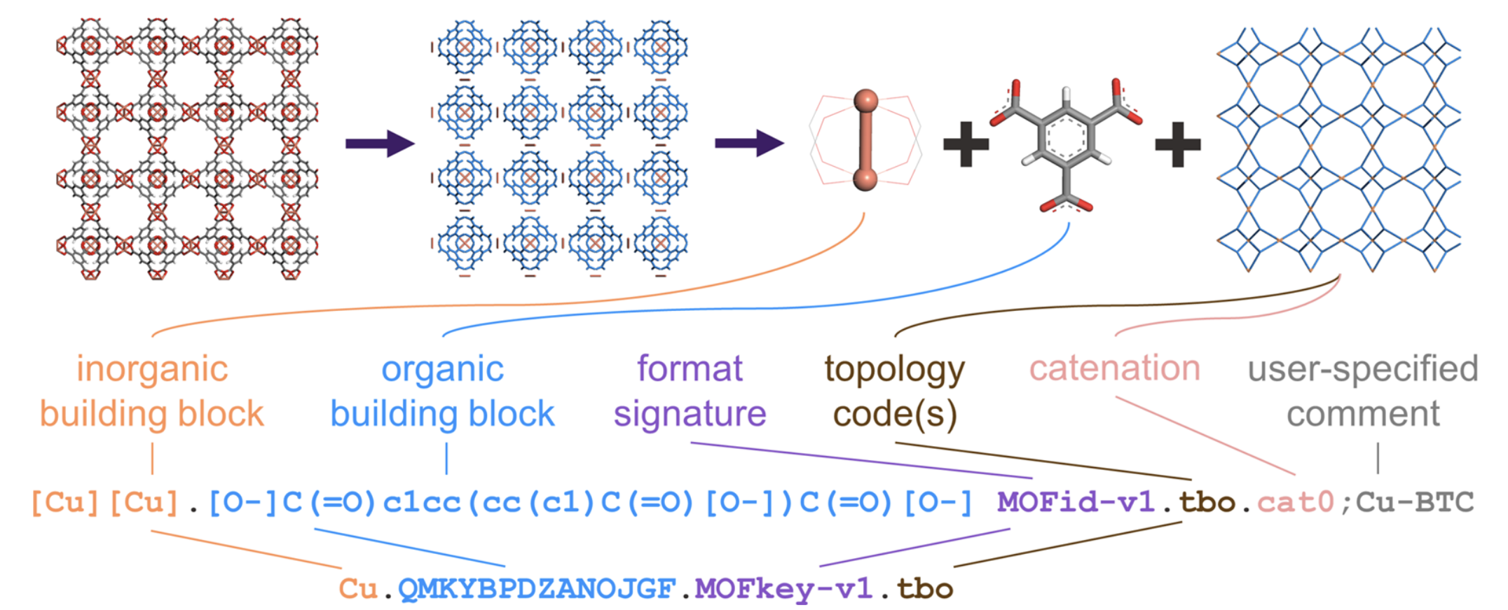
In prior work by Bucior et al., a pair of methods known as MOFid and MOFkey are described that can be used to assign a unique name for a given MOF. MOFid works by deconstructing a MOF into its node(s), linker(s), and topology. The nodes and linkers are represented as SMILES strings, the topology is determined using Systre, and any catenation is noted. These factors are combined into a single unique "MOFid". The MOFkey is simply a shorter, InChI-based hash of the MOFid. These methods are shown below for HKUST-1 (also known as Cu3(btc)2 and Cu-BTC):

The MOFid code is available here with a web-based version available here.

The SMILES search on the MOF Explorer is a partial-match of the MOFid. As such, one can query by just the node, just the linker, or even a substructure of the linker. If the user wishes to supply both a node and linker query, they should be provided in the MOFid format (separated by a "." with the node(s) listed before the linker(s)).

All partial atomic charges are computed at the PBE-D3(BJ) geometry using one of several population analysis methods: Bader, DDEC6, and CM5. The DDEC6 and CM5 charges were calculated from Chargemol 09-26-2017. In all cases, the partial atomic charges are calculated from the DFT-computed charge density. In the QMOF Database, partial atomic charges are calculated using a charge density at one of four several levels of theory: PBE, HLE17, HSE06*, and/or HSE06. In general, the different levels of theory predict similar partial atomic charges. The different charge partitioning schemes, however, can result in very different partial atomic charges.

We report multiple magnetic properties for each material, including a net magnetic moment, atomic magnetic moments from VASP, and atomic spin densities calculated using the Bader and DDEC6 methods. In general, a high-spin magnetic initialization was provided (similar to what is done for the Materials Project). We note, however, that this does not mean all materials have high-spin character, as the initial magnetic moments are adjusted until they converges to a local minimum energy configuration in VASP. For applications that are highly reliant on an accurate description of the magnetic character, we acknowledge that there may be a lower energy magnetic configuration not captured via this initialization procedure.

Bond orders were computed using the method. Bond orders displayed in the MOF Explorer are the effective bond orders for each atom (i.e. a single value representing the sum of bond orders between the atom of interest and its neighbors). For the full list of bond orders between every pair of atoms, we refer the user to the DDEC6 files made available on NOMAD. For the crystal structure visualization, bond orders are not taken into account; instead, the coordination environments are determined from Pymatgen's .

In this section, we will review how to use the Catalysis Explorer app of the Materials Project. The Catalysis Explorer allows for visualising structures with surface adsorbates and provides adsorption energies for those structures.

1. Go to Materials Project - Catalysis Explorer

To begin, click the above link to go to the Catalysis Explorer app.

2. Search by composition

One of the ways of searching for a particular surface is through the bulk formula, within the composition tab. For example, you could search for Ti2Pd3.

3. Search by Adsorbate

Choose a certain adsorbate based on the SMILES or IUPAC formula. For example, if you were interested in finding the adsorption energy for CH2, the adsorbate SMILES would be *CH2 and the IUPAC formula would be C1 H2.

5. Search by formula

In this tab, you can choose surfaces based on their formula, material ID corresponding to their bulk, miller indices of the surface (individually as h,k,l) and surface shifts.

6. Real example

Say we were interested in CH2* on Ti2Pd3. Input the options in points 2 and 3 of this tutorial to find the following search results from the database (note that the exact options might change in the future).

7. Visualize structure and adsorption energies

Components

Search

You can search using the periodic table to select different elements you would like in your Pourbaix diagram. You can select up to 4 elements to build the Pourbaix diagram.

Advanced Options

Several advanced opttions are available. You can filter solids, display a heatmap, or change the composition.

Pourbaix Diagram Viewer

Citations

To cite the Pourbaix Diagram App on Materials Project, please include the main Materials Project citation, as well as the references below:

Patel, Anjli and Norskov, Jens and Persson, Kristin and Montoya, Joseph. Efficient Pourbaix diagrams of many-element compounds, Physical Chemistry Chemical Physics 45 (2019)

Singh, Arunima and Zhou, Lan and Shinde, Aniketa and Suram, Santosh and Montoya, Joseph and Winston, Donald and Gregoire, John and Persson, Kristin. Electrochemical Stability of Metastable Materials, Chemistry of Materials 29 (2017)

Persson, Kristin and Waldwick, Bryn and Lazic, Predrag and Ceder, Gerbrand. Prediction of solid-aqueous equilibria: Scheme to combine first-principles calculations of solids with experimental aqueous states, Physical Review B 85 (2012)

How to Cite

If you use the MOF Explorer in your work, please cite the following two references:

1. A.S. Rosen, S.M. Iyer, D. Ray, Z. Yao, A. Aspuru-Guzik, L. Gagliardi, J.M. Notestein, R.Q. Snurr. "Machine Learning the Quantum-Chemical Properties of Metal–Organic Frameworks for Accelerated Materials Discovery", Matter, 4, 1578-1597 (2021). DOI: .

2. A.S. Rosen, V. Fung, P. Huck, C.T. O'Donnell, M.K. Horton, D.G. Truhlar, K.A. Persson, J.M. Notestein, R.Q. Snurr. "High-Throughput Predictions of Metal–Organic Framework Electronic Properties: Theoretical Challenges, Graph Neural Networks, and Data Exploration," npj Comput. Mat., 8, 112 (2022). DOI: .

Ref. 1 describes the original release of the Quantum MOF (QMOF) Database, which at the time of publication consisted of PBE-computed properties for ~14,000 MOFs. This is the primary reference for the QMOF Database.

Ref. 2 builds upon the QMOF Database by introducing the MOF Explorer application, raises the number of structures to ~20,000, introduces hypothetical MOFs to the QMOF Database, and supplements the PBE data with HLE17, HSE06*, and HSE06 static calculations for select materials.

In addition, if using the data in your own work, we recommend specifying the version number for reproducibility purposes. The current version number is included at the bottom of each MOF details page and corresponds to the current version of the QMOF Database on .

What input file formats are supported?

Any input file format supported by pymatgen. This includes CIF, POSCAR, CSSR and pymatgen JSON. See here for more information. Additional file formats might be supported on request.

A transformation doesn't seem to be working?

Please ask on the if this is a problem for you. We are improving this functionality over time. For advanced users, all transformations are also available for use via .

The Molecules Explorer app is a new feature of the Materials Project. It enables searching for molecules relevant for electrolyte applications. The API is similar to that of Materials Explorer, where the user can query by one of the following methods:

• Elements only;

• Chemical formula;

• SMILES string;

• Molecule ID.

Upon receiving the query, Molecules Explorer outputs the search result, including information of the relevant molecules based on the query. For each molecule, the following properties are provided:

• Electron Affinity;

• Ionization Energy;

• SMILES string representation;

In this section, we present several ways to navigate through the Battery Explorer.

The Battery Explorer app allows users to filter candidate battery materials using chemical formula/composition, as well as properties such as maximum volume change, average voltage, capacity, stability etc.

In each individual page for a battery material, the user can find information regarding the material such as calculated properties, voltage curve, oxygen evolution graph and a visulization of the host material.

1.

Downloading the QMOF Database

The recommended way of downloading much of the data underlying the QMOF Database is at the following Figshare repository: . The data on Figshare includes DFT-optimized geometries (in XYZ and CIF format) and several tabulated properties, such as energies, partial atomic charges (DDEC6, CM5, Bader), bond orders (DDEC6), atomic spin densities (DDEC6, Bader), magnetic moments, band gaps, and more. For reproducibility purposes, we recommend noting the version of the QMOF Database you have used. Note that a mirror of the QMOF Database made to be interoperable with the Materials Project is available on , which can be queried with the if desired.

Introduction

Surface energy is a measure of the energy change associated with the breaking of intermolecular bonds in a bulk material to create a surface. In thermodynamically stable materials, the creation of a surface will always increase energy, otherwise there would be a thermodynamic driving force to create surfaces and the material would sublimate. In theory, surface energy is equal to half of the energy of cohesion (the energy needed to break all of the bonds required to form two new surfaces). However, this perfect cleaving of surfaces is rarely achieved. In reality, surfaces often rearrange and/or react with their surroundings to passivate or adsorb molecules or atoms to lower their surface energy from the theoretical cohesive energy value.

Basic search for a material in the MP database

1. Go to Materials Project - Materials Explorer

2. Type the search criteria such as the composition, chemical formula or mp-id in the search box or click the elements from the periodic table below the search box

3. Use the filters in the left to filter the search results

4. Click on Search

5. Click on Columns to select what properties to show for the search results

6. Click on the mp-id to go to the material page

7. Use the right tool bar on the to change the visualization settings and export the structure file

8. To download the structure, click "Export as"

9. A summary of material properties is shown in the right

10. An auto-generated description of the material from generated using Robocrystallographer (https://github.com/hackingmaterials/robocrystallographer)

11. Click on Crystal Structure to look at the basic structure information

12. Click on Properties to look at the materials properties

See the Methodology section for how these properties were calculated

The Phase Diagram App allows a user to create and visualize compositional phase diagrams for 1, 2, 3, and 4 element chemical systems using Materials Project data. It is also possible to create and visualize the corresponding chemical potential diagrams for 2 and 3 element systems. The user has access to some customization features, such as 1) changing the style of plot, 2) selecting data calculated with a certain DFT functional, 3) and using machine learning (ML)-estimated finite temperature data.

Methodology

The methodology behind thermodynamic energy calculations, phase diagram construction, and chemical potential diagram construction has been extensively discussed in the Methodology section of the MP Docs. See the links below:

App Components

Search by chemical system

Phase diagrams are created by chemical system (i.e., a collection of elements). To create a phase diagram in the Phase Diagram App, first select a set of elements by typing them either as a single string separated by dashes, or by clicking the elements in the periodic table viewer (which will auto-populate the search box).

Visualization Viewer

Once a chemical system has been selected (e.g., Li-Fe-O), you will an illustration of the compositional phase diagram for your system of interest load in the the viewer. Within the viewer, you can switch to the chemical potential diagram to view the same phase equilibria but within chemical potential space (see for more information).

1) Phase Diagram

2) Chemical Potential Diagram

If you are

Configure Visualization

The phase diagram viewer can be configured

Advanced Options

Data Table

MPContribs provides a platform and advanced programming interface (API) to contribute computational as well as experimental data to Materials Project. Data on MPContribs is collectively maintained as annotations to existing MP materials (or formulas and chemical systems), and automatically exposed to over 200,000 MP users. The platform serves as the backbone for data and apps contributed to MP while leaving full ownership and control over the data with contributors. Contributed data is automatically shown on MP's or its disambiguation pages for formulas and chemical systems. A dedicated landing page is provided for each MPContribs project which can be used to reference the dataset in journal publications through Digital Object Identifiers (DOIs) provided by MP in collaboration with the DOE Office of Scientific and Technological Information (). The MPContribs can be used to programmatically retrieve, upload and modify contributed data.

See below for a list of and an overview of its . Continue with the following sections in MP's documentation to learn more:

Introduction

Materials synthesis techniques such as Chemical Vapor Deposition, Molecular Beam Eptixay, Sputtering, etc. are prevalent in materials research. Synthesizing materials with these techniques comes with a challenge: how does one determine which subtrate to use?

Epitaxial growth of heterogeneous interfaces requires a fundamental understanding of the substrate material, film material, cleavage planes, lattice mismatches, and resultant stresses and strains. The Materials Project (MP) stores crystallographic information for each material in its database, calculated via First Principles Density Functional Theory. Each material's crystallographic information, in particular the surface termination lattice parameters, is especially useful to find the epitaxial matches between a desired material (film) and a corresponding substrate. The Suggested Substrates tool outputs the Miller Indices of the substrate and the film (target material) termination plane, the minimal co-incident area (MCIA), and Elastic Energy.

Introduction

A phonon is a collective excitation of a set of atoms in condensed matter. These excitations can be decomposed into different modes, each being associated with an energy that corresponds to the frequency of the vibration. The different energies associated with each vibrational mode constitute the phonon vibrational spectra (or phonon band structure). The vibrational spectra of materials play an important role in physical phenomena such as thermal conductivity, superconductivity, ferroelectricity and carrier thermalization.

There are different methods to calculate the vibrational spectra from first-principles using the density functional theory formalism (DFT). It can be obtained from the Fourier transform of the trajectories of the atoms on a molecular dynamics run, from finite-differences of the total energy with respect to atomic displacements or directly from density functional perturbation theory (DFPT). The latter method is the one used in the calculations on the Materials project page.

1.

1.

1. Visit ;

2. On the crystal toolkit web page, one can query Materials Project by MP-ID, or upload a structure file. (of what format???)

3. The interactive graphic user interface allows the user to visualize and manipulate crystal structures.

Calculation Details

A relaxed structure associated with the canonical data in the entries field of a material data entry is used to run both uniform and line-mode NSCF calculations with the same functional (and U if any). Currently, only GGA (PBE) and GGA+U DOS and band structures are available from the database.

We first run a static (SCF) calculation with a uniform (Monkhorst Pack or $\Gamma$-centered for hexagonal systems) k-point grid determined by the standard MPStaticSet input set in pymatgen. The charge density is extracted from this and used for the subsequent uniform and line-mode NSCF calculations. The parameters for both of these are determined by the MPNonSCFSet input set in pymatgen. For more details, see the band structure workflow in .

Line-mode Band Structure

The line-mode NSCF calculation is run with k-points chosen along high-symmetry lines within the Brillouin zone of the material. Currently, three conventions for choosing this k-path are used, and follow the methodologies by Curtarolo et al. , Hinuma et al. , and Munro et al. Code for generating the k-paths can be found within .

The Setyawan-Curtarolo band structure data is displayed on the website by default with full lines for spin-up and dashed lines for spin-down. For insulators, the band gap is computed according to the band structure. The nature of the gap (direct or undirect) as well as the k-points involved in the band gap transition are displayed. The VBM and CBMs are displayed for insulators as well by purple dots. Note that the website might not show all bands included in the calculation. These can be obtained by by downloaded the band structure data from the .

Density of States (DOS)

The DOS displayed on the website shows the total DOS, and elemental projections by default. However, total orbital and elemental orbital projections are also calculated and available from the . Please note that the DOS data and line-mode band structure may not completely agree on all derived properties such as the band-gap due to k-point grid differences. For instance, the uniform k-point grid used to calculate the DOS might not include some specific k-points along one of the high-symmetry lines, while the line-mode band structure will.

Material Band Gap

The band gap listed for a given material is chosen from one of its calculations. The current calculation hierarchy is as follows:

Density of States > Line-mode Band Structure > Static (SCF) > Optimization

Accuracy of Band Structures

Note: The term 'band gap' in this section generally refers to the fundamental gap, not the optical gap. The difference between these quantities is reported to be small in semiconductors but significant in insulators.

Figure 1: Experimental versus computed band gaps for 237 compounds in an internal test. The computed gaps are underestimated by an average factor of 1.6, and the residual error even after accounting for this shift is significant (MAE of 0.6 eV). We thank M. Chan for her assistance in compiling this data.

Density functional theory is formulated to calculate ground state properties. Although the band structure involves excitations of electrons to unoccupied states, the Kohn-Sham energies used in solving the DFT equations are often interpreted to correspond to electron energy levels in the solid.

The correspondence between the Kohm-Sham eigenvalues computed by DFT and true electron energies is theoretically valid only for the highest occupied electron state. The Kohn-Sham energy of this state matches the first ionization energy of the material, given an exact exchange-correlation functional. However, for other energies, there is no guarantee that Kohn-Sham eigenvalues will correspond to physical observables.

Despite the lack of a rigorous theoretical basis, the DFT band structure does provide useful information. In general, band dispersions predicted by DFT are reported to match experimental observations; one small test of band dispersion accuracy found that errors ranged from 0.1 to about 0.4 eV. However, predicted band gaps are usually severely underestimated. Therefore, a common way to interpret DFT band structures is to apply a 'scissor' operation whereby the conduction bands are shifted in energy by a constant amount so that the band gap matches known experimental observations.

Band gaps

In general, band gaps computed with common exchange-correlation functionals such as the LDA and GGA are severely underestimated. Typically the disagreement is reported to be around 50% in the literature. Some internal testing by the Materials Project supports these statements; typically, we find that band gaps are underestimated by about 40% (Figure 1). We additionally find that several known insulators are predicted to be metallic.

Origin of band gap error and improving accuracy

The errors in DFT band gaps obtained from calculations can be attributed to two sources: 1. Approximations employed to the exchange correlation functional 2. A derivative discontinuity term, originating from the true density functional being discontinuous with the total number of electrons in the system.

Of these contributions, (2) is generally regarded to be the larger and more important contribution to the error. It can be partly addressed by a variety of techniques such as the GW approximation but typically at high computational cost.

Strategies to improve band gap prediction at moderate to low computational cost now been developed by several groups, including Chan and Ceder (delta-sol), Heyd et al. (hybrid functionals) , and Setyawan et al. (empirical fits) . (These references also contain additional data regarding the accuracy of DFT band gaps.) The Materials Project may employ such methods in the future in order to more quantitatively predict band gaps. For the moment, computed band gaps should be interpreted with caution.

Citation

To cite the calculation methodology, please reference the following works:

1. A. Jain, G. Hautier, C. Moore, S.P. Ong, C.C. Fischer, T. Mueller, K.A. Persson, G. Ceder., A High-Throughput Infrastructure for Density Functional Theory Calculations, Computational Materials Science, vol. 50, 2011, pp. 2295-2310.

Authors

1. Anubhav Jain

2. Shyue Ping Ong

3. Geoffroy Hautier

References

[1]: W. Setyawan, S. Curtarolo, High-throughput electronic band structure calculations: Challenges and tools, Computational Materials Science 2010, 49, 299-312.

[2]: Y. Hinuma, P. Giovanni, Y. Kumagai, F. Oba, I. Tanaka, Band structure diagram paths based on crystallography Computational Materials Science 2017, 128, 140-184.

[3]: J.M. Munro, K. Latimer, M.K. Horton, S. Dwaraknath, K.A. Persson, An improved symmetry-based approach to reciprocal space path selection in band structure calculations, npj Computarional Materials 2020, 6, 112.

[4]: E.N. Brothers, A.F. Izmaylov, J.O. Normand, V. Barone, G.E. Scuseria, Accurate solid-state band gaps via screened hybrid electronic structure calculations., The Journal of Chemical Physics. 129 (2008)

[5]: R. Godby, M. Schluter, L.J. Sham, Self-energy operators and exchange-correlation potentials in semiconductors, Physical Review B. 37 (1988).

[6]: M. Chan, G. Ceder, Efficient Band Gap Predictions for Solids, Physical Review Letters 19 (2010)

[7]: J. Heyd, J.E. Peralta, G.E. Scuseria, R.L. Martin, Energy band gaps and lattice parameters evaluated with the Heyd-Scuseria-Ernzerhof screened hybrid functional, Journal of Chemical Physics 123 (2005)

[8]: W. Setyawan, R.M. Gaume, S. Lam, R. Feigelson, S. Curtarolo, High-throughput combinatorial database of electronic band structures for inorganic scintillator materials., ACS Combinatorial Science. (2011).

Introduction

Piezoelectricity is a reversible physical process that occurs in some materials whereby an electric moment is generated upon the application of a stress. This is often referred to as the direct piezoelectric effect. Conversely, the indirect piezoelectric effect refers to the case when a strain is generated in a material upon the application of an electric field. The mathematical description of piezoelectricity relates the strain (or stress) to the electric field via a third order tensor. This tensor describes the response of any piezoelectric bulk material, when subjected to an electric field or a mechanical load.

The piezoelectric constants from the Materials Project (MP) are calculated from first principles Density Functional Perturbation Theory (DFPT) [1] and are approximated as the superimposed effect of an electronic and ionic contribution. From the full piezoelectric tensor, several properties are derived such as the maximum longitudinal piezoelectric modulus and the corresponding crystallographic direction. Just as with the elastic constants, multiple consistency checks are performed on all the calculated piezoelectric data to ensure its reliability and accuracy.

Figure 1: longitudinal piezoelectric modulus-surface for a cubic compound, showing the maximum response in the <111> family of directions.

Formalism

In this work, we calculate the piezoelectric stress coefficients, from DFPT, with units of . These can be defined in terms of thermodynamic derivatives as shown below .

where , , , and represent the electric displacement field, the electric field, the strain tensor, the stress tensor and the temperature, respectively.

The above relations can be written in Voigt-notation as shown below.

We note that the most commonly used piezoelectric constants appearing in the (experimental) literature are the piezoelectric strain constants, usually denoted by . These can be readily related to the constants if the elastic compliances (at constant electric field and temperature) of the materials are known: . In particular, the piezoelectric strain constants can be expressed thermodynamically as shown below

It is well-known that the piezoelectric behavior can only occur in crystals that lack inversion symmetry. This is the direct consequence of the symmetry properties of the piezoelectric tensor, which is of order 3. Another fundamental requirement for piezoelectric behavior is that the material has a band gap. Combined, these criteria severely limit the amount of compounds in nature that have the potential to exhibit piezoelectric behavior.

For the Materials Project in particular, potential piezoelectric materials in the database are identified by i) allowing only structures with space groups 1, 3-9, 16-46, 75-82, 89-122, 143-146, 149-161, 168-174, 177-190, 195-199, 207-220 (since these space groups lack inversion symmetry), and in addition ii) the calculated DFT bandgap of the material > 0.1 eV. Compounds in the Materials Project database that satisfy these criteria are selected for a full-DFT calculation of the piezoelectric tensor and derived properties (see below).

Derived piezoelectric properties

For elastic properties, which are based on a tensor of order 4, isotropic Voigt and Reuss averages can be derived on the bulk and shear moduli. For piezoelectric properties, this isotropic averaging-approach does not quite work due to the requirement that inversion symmetry cannot occur in piezoelectric materials. On MP, in addition to the piezoelectric tensor in Voigt-notation, we report the maximum longitudinal piezoelectric modulus of the compound and the corresponding crystallographic direction in which this occurs. One can think of these quantities as the piezoelectric counterpart of the well-known Young's modulus and the stiffest elastic direction in the context of elasticity-theory. Fig. 1 shows an example of how the longitudinal piezoelectric modulus can be represented in 3D. This is for the case of a cubic material. As can be seen clearly, the maximum modulus occurs in the <111> family of crystallographic directions. By symmetry, this is always the case for cubic piezoelectric materials. Fig. 2 shows a more complicated longitudinal piezoelectric modulus-surface for an orthorhombic compound. In that case, the relative magnitudes of the tensor components dictate in which crystallographic direction, the maximum response occurs. Finally, note that for some compounds, a piezoelectric response is only induced by shear deformation rather than tensile or compressive deformation. For these cases, the response cannot be depicted such as in Figs. 1 and 2. The representations such as in Figs. 1 and 2 and created using the open-source MTEX package .

Figure 2: longitudinal piezoelectric modulus-surface for an orthorhombic compound.

DFT parameters

The first-principles results presented in this work are performed using the projector augmented wave (PAW) method as implemented in the Vienna Ab Initio Simulation Package (VASP). In all calculations, we employ the Perdew, Becke and Ernzerhof (PBE) Generalized Gradient Approximation (GGA) for the exchange-correlation functional. A cut-off for the plane waves of 1000 eV is used and a uniform k-point density of approximately 2,000 per reciprocal atom (pra) is employed, which means that the number of atoms per cell multiplied by the number of k-points equals approximately 2,000. For the compounds that contain magnetic elements, a ferromagnetic state is initialized in the calculation. Similarly to our previous work, we expect to correctly converge to ferromagnetic and non-magnetic states in this way, but not to anti-ferromagnetic states. Due to the presence of strongly correlated electrons in some of the oxides, the GGA+U method is employed, with U representing the Hubbard-parameter. The values of U are chosen consistent with those employed in MP.

Figure 3: A graphical representation of the piezoelectric dataset, currently containing over 900 materials. A series of concentric circles indicate constant values of the maximum longitudinal piezoelectric modulus, . The compounds are broken up according to the crystal system and the different point group symmetry-classes considered in this work. See the paper for details.

Crystal symmetry

The crystal symmetry and in particular the point group dictates the symmetry of the piezoelectric tensor, relates components of the tensor to each other and imposes that certain components equal zero. All piezoelectric tensors in the Materials Project have been symmetrized for consistency with the underlying point group of the compound. Figure 4 gives an overview of the symmetrized piezoelectric tensors in MP, broken up by the different piezoelectric point groups. Also, typical surface representations are shown. The point group that only yields piezoelectric behavior upon the application of shear is not included in the representation in Fig. 4.

Figure 4: Piezoelectric tensors and symmetry classes considered in this work. Typical representations of the longitudinal piezoelectric modulus in 3D are also shown for each crystal point group. Note that depending on the components of the piezoelectric tensor, the surface representation can differ from those shown here. See the paper for details.

Citation

To cite the piezoelectric properties within the Materials Project, please reference the following work:

• de Jong, Maarten and Chen, Wei and Geerlings, Henry and Asta, Mark and Persson, Kristin Aslaug. A database to enable discovery and design of piezoelectric materials,

The paper presents the results of our piezoelectric constant-calculations for the first batch of 941 compounds. Our DFT-parameters, the workflow and comparison to experiments are described in detail. Also, the filters in the workflow used for detecting anomalies in the calculations are described in the paper.

Authors

1. Maarten de Jong

References

[1]: Baroni, Giannozzi S. P. and Testa, A. Phys. Rev. Lett. 58, 1861 (1987)

[2]: Nye, J. F. Physical properties of crystals (Clarendon press, 1985).

[3]: Bachmann, F., Hielscher, R. & Schaeben, H. Texture analysis with MTEX-free and open source software toolbox. Solid State Phenomena 160, 63–68 (2010).

[4]: Hielscher, R. & Schaeben, H. A novel pole figure inversion method: specification of the MTEX algorithm. Journal of Applied Crystallography 41, 1024–1037 (2008).

[5]: Mainprice, D., Hielscher, R. & Schaeben, H. Calculating anisotropic physical properties from texture data using the MTEX open-source package. Geological Society, London, Special Publications 360, 175–192 (2011).

Each material in the QMOF Database, and thereby the MOF Explorer, was taken from an existing dataset of MOF structures. Some of these datasets are dedicated to experimentally synthesized MOF structures, whereas others are hypothetical MOF structures (i.e. computationally constructed). Below, we outline the various datasets of MOF structures used in constructing the QMOF Database.

Cambridge Structural Database – MOF Subset

The Cambridge Structural Database (CSD) contains experimentally derived crystal structures for over a million materials. Of the crystal structures published on the CSD, approximately 100,000 are included in what is referred to as the CSD MOF Subset. It should be noted that the definition of a MOF in the CSD MOF Subset is more inclusive than many other databases and includes non-porous materials that are arguably best described as coordination polymers, in addition to more conventional MOF structures.

In the QMOF Database, structures were taken directly from the CSD MOF Subset with free (i.e. unbound) solvent removed from the pores. was used to download the structures, and we excluded materials that were flagged as having charge-balancing ions, any errors in the crystal structure, or disorder in the framework. Additionally, we excluded any structures that lacked carbon or hydrogen atoms, had atoms with close interatomic distances, had lone (i.e. unbonded) atoms, or had terminal oxo ligands on metals where such ligands are typically OH groups or water. Several scripts to carry out these fidelity checks can be found .

CoRE MOF Database

The contains experimentally derived crystal structures for ~14,000 porous, three-dimensional MOFs. The materials in the CoRE MOF Database were derived from the CSD but are not directly associated with the CSD MOF Subset, although many of the CoRE MOFs can be found in the CSD MOF Subset as well. Unlike the CSD MOF Subset, which provides as-reported crystal structures, a suite of automated and manual structural corrections were carried out during the construction of the CoRE MOF Database. As with any automated approach, not all of these structural corrections are perfect in their execution and can result in materials with misplaced atoms, under- and over-bonded atoms, charge imbalances, and similar structural fidelity issues that can be determinetal for DFT.

In the QMOF Database, we considered CoRE MOFs that were included in curated lists provided by and to increase the likelihood of having high-fidelity CoRE MOF structures. For consistency, the free solvent-removed (FSR) subset of the CoRE MOF Database was conisdered. We emphasize that there are many MOFs present in the CoRE MOF Database that we instead adopted from the CSD MOF Subset directly. As such, if a user is specifically interested in which MOFs in the QMOF Database are also present in the CoRE MOF Database, one should compare the CSD reference codes and/or MOFids for the materials in these two datasets.

Pyrene MOFs

Several experimentally characterized, pyrene-containing MOFs were taken from the work of using the structures that were uploaded to the . No further modifications were made to these structures.

ToBaCCo

The can generate hypothetical MOFs from known inorganic and organic building blocks (and topologies). Here, the "ToBaCCo" dataset of MOFs specifically refers to those found in the by Colón, Gómez-Gualdrón, and Snurr. In the QMOF Database, MOFs with triangular Cu-containing nodes were selected from the ToBaCCo dataset, as found .

Anderson and Gómez-Gualdrón

The contains hypothetical MOFs constructed using ToBaCCo. In the QMOF Database, we selected Zr-containing MOFs from this dataset. We also expanded the dataset to include hypothetical Hf-containing MOfs by exchanging the Zr species for Hf.

Boyd & Woo

Hypothetical MOFs in the QMOF Database were also adopted from the work of using the dataset of structures uploaded to the Materials Cloud . These MOFs were construced using the , as described in prior work by . As a result, we refer to these hypothetical MOFs as coming from the Boyd & Woo dataset.

In the QMOF Database, we adopted MOFs from select families in the Boyd & Woo daaset and occasionally made modifications to several of these MOFs to diversify our collection. For instance, we occasionally exchanged the metals in the inorganic node, and we constructed Al rod MOFs by exchanging the metals in the pre-existing V rod MOFs and protonating the bridging oxo ligands. We still refer to these structures as being derived from the Boyd & Woo dataset even though custom modifications have been made.

Genomic MOF Database

Hypothetical MOFs from the made available were included in the QMOF Database. These structures were adopted as-is without further modification.

Mail-Order MOF-5s

Hypothetical MOF-5 analogues were obtained from by Haranczyk and colleagues. See for the dataset.

Hypothetical MOF-74s

Hypothetical Mg-MOF-74 analogues were obtained from by Haranczyk and colleagues.

Introduction

A dielectric is a material that can be polarized by an applied electric field. This limits the dielectric effect to materials with a non-zero band gap. The mathematical description of the dielectric effect is a tensor constant of proportionality that relates an externally applied electric field to the field within the material. Along with the elastic and piezoelectric tensors, the dielectric tensor provides all the information necessary for the solution of the constitutive equations in applications where electric and mechanical stresses are coupled.

The dielectric tensors from the Materials Project (MP) are calculated from first principles Density Functional Perturbation Theory (DFPT) and are approximated as the superimposed effect of an electronic and ionic contribution. From the full piezoelectric tensor, several properties are derived such as the refractive index and potential for ferroelectricity. Just as with the piezoelectric and elastic constants, multiple consistency checks are performed on all the calculated dielectric data to ensure its reliability and accuracy.

References

[1]: Ong, S. P. et al. Python Materials Genomics (pymatgen): A robust, open-source python library for materials analysis. Computational Materials Science68, 314–319 (2013)
[2]: Tran, R., Xu, Z., Radhakrishnan, B. et al. Surface energies of elemental crystals. Sci Data3, 160080 (2016)
γhklσ=2⋅AslabEslabhkl,σ−Ebulkhkl⋅nslab
2. Search the chemical formula of interest
Step 2 screenshot
3. Choose the filter of choice under the "Composition" Tab on the left
Step 3 screenshot
4. Select the working ion of choice
Step 4 screenshot
5. One can delete filters by clicking "x" next to the filter
Step 5 screenshot
6. Try a different type of filtering requirement - chemical system
Step 6 screenshot
7. Under Battery Properties tab on the left, choose filter of choice
Step 7 screenshot
8. Filter by average voltage
Step 8 screenshot
9. Filter by stability of the discharged state
Step 9 screenshot
10. Change the x-axis for the voltage curve
Step 10 screenshot
11. Link to materials detail page for each voltage step
Additional files and properties beyond those hosted on Figshare (e.g. VASP inputs and outputs, density of states, charge densities) can be obtained from NOMAD and Globus, as described in more detail below.
Downloading the VASP Files
NOMAD
All VASP input and output files are made available on NOMAD at the following datasets:
Querying NOMAD by external_id will allow you to search by the unique QMOF ID available on the MOF Explorer. Including a supplemental query of datasets will allow the user to specify one of the four datasets listed above for a specified level of theory. Links to the NOMAD files for a given material are available on each material's detail page. See the "Calculation Parameters" section of the documentation for a description of the different levels of theory.
Please note that there may be more entries on NOMAD than in the MOF Explorer. This is because structures are occasionally removed from the QMOF Database if any structural fidelity issues are identified, but entries cannot be deleted from NOMAD.
To download an entire NOMAD dataset, switch from the default "Entries" view to "Datasets".
Globus - Charge Densities
Due to their large filesizes, charge densities are made available via a Globus endpoint. First, set up a collection end-point, which can include your local machine or a compute cluster with Globus installed. Then choose a path in the collection in which to store the files. Once this is set up, select the folders and/or files you wish to download from the QMOF collection and choose "Transfer or Sync to..." to have Globus transfer the files to your specified location.
[1]: Gonze, X. & Lee, C. Dynamical matrices, Born effective charges, dielectric permittivity tensors, and interatomic force constants from density functional perturbation theory. Phys. Rev. B 55, 10355–10368 (1997)
[2]: C. Lee & X. Gonze, Ab initio calculation of the thermodynamic properties and atomic temperature factors of SiO2 α-quartz and stishovite. Phys. Rev. B 51, 8610 (1995)
[3]: Gonze, X. et al. First-principles computation of material properties: the Abinit software project. Computational Materials Science 25, 478 – 492 (2002)
[4]: Gonze, X. et al. ABINIT: First-principles approach to material and nanosystem properties. Computer Physics Communications 180, 2582 – 2615 (2009)
[5]: Perdew, J. P. et al. Restoring the density-gradient expansion for exchange in solids and surfaces. Phys. Rev. Lett. 100, 136406 (2008)
[6]: He, L. et al. Accuracy of generalized gradient approximation functionals for density-functional perturbation theory calculations. Phys. Rev. B 89, 064305 (2014)
[7]: Hamann, D. R. Optimized norm-conserving Vanderbilt pseudopotentials. Phys. Rev. B 88, 085117 (2013)
[8]: van Setten, M., Giantomassi, M., Bousquet, E., Verstraete, M.J., Hamann, D.R., Gonze, X. & Rignanese, G.-M., et al. The PseudoDojo: Training and grading a 85 element optimized norm-conserving pseudopotential table (2018). Computer Physics Communications 226, 39.
[9]: Petretto, G., Gonze, X., Hautier, G. & Rignanese, G.-M. Convergence and pitfalls of density functional perturbation theory phonons calculations from a high-throughput perspective. Computational Materials Science 144, 331 – 337 (2018)
[10]: Setyawan, W. & Curtarolo, S. High-throughput electronic band structure calculations: Challenges and tools. Computational Materials Science 49, 299 – 312 (2010)
The table below lists the various MPContribs portals currently available. When you explore data or consider contributing your data to MP, please pick the portal that best aligns with it.
Portal
URLs
Description
MPContribs
Datasets that don't fall under the purview of the other portals
MPContribsML
Benchmark datasets for Machine Learning
Concepts
Each MPContribs deployment is organized into projects. The MP account creating the project becomes its owner. An owner can ask for the MP accounts of their collaborators to be given access to their project. A collaborator assumes the same level of permissions within a project as the owner.
A project contains a list of contributions to existing MP materials (or alternatively to formulas and chemical systems). It's in the owner's purview to decide what exactly constitutes a project. Often this will simply be an umbrella for a dataset containing contributions to MP materials that are comparable in their scientific context and thus are consistent in their data schema.
Any MP account can create (or be an owner of) a maximum of 3 projects at any time. Project owners can immediately start adding up to 500 contributions to their project without approval from MP. To add more contributions, project owners or their collaborators can reach out to MPContribs administrators to obtain approval.
By default, projects are set to private, i.e. only visible to owners and their collaborators. Each individual contribution in a project is set to public by default and thus automatically released to the public when the project is published. Since the public/private flag can be controlled for each contribution individually, some contributions in a project can be kept private even if the project is public. The public/private state of a project and its contributions can be changed/reverted at any time.
A single contribution constitutes a small blob of data assigned and linked to the according MP material through identifiers such as MP's materials IDs, formulas or chemical systems. In addition to these identifiers, each individual contribution can contain the following four components:
A data component containing hierarchically organized key-value data (think nested dictionaries). In its flattened format, this component can contain a maximum of 50 keys/fields each of which becomes a column in the overview table on the project landing pages. Nested fields in the data dictionary are organized as nested columns on the landing page table. Any data types included in the data component become queryable, filterable and sortable using a wide variety of operators. Also see the API documentation for any MPContribs deployment for a generic list of available filters.
A structures component containing a list of up to 10 pymatgen structures with optionally customized names. A string in the format used for Crystallographic Information Files (CIFs) is stored with each structure and can be retrieved through the API or downloaded through the project landing pages.
A tables component containing a list of up to 10 . This component is intended for the inclusion of 2D spectra (think CSV files) with each contribution. A is generated for each table and included in the according contribution detail page for visualization purposes. Each DataFrame's name and other attributes (title, axis labels, ...) needed to configure the Plotly graph can be controlled via the Dataframes' attrs attribute. The total number of table rows is stored and all table cells formatted automatically. The API paginates the table rows for more efficient data retrieval. Each table can be downloaded as CSV programmatically or through the project landing pages.
An attachments component containing a list of up to 10 with customized names. Attachments can be gzipped text files (CSV, JSON, ...) or images in PNG, JPEG, GIF, or TIFF formats. An attachment can either be created directly from a file path or from a python list or dictionary using the mpcontribs.client.Attachment.from_data() method. Each attachment can be up to 2.4 MB large. Attachment meta-data are queryable but not its contents (think e-mail attachments).
Duplicate structures, tables, and attachments are only saved once internally but referenced by all contributions they were submitted with. See the section about contributing data for more information and examples.
Suggested Substrates tool in MP relies mainly on the geometrical principles of lattice matching, based off of Zurr and McGill [1].
Suppose there is two slabs of materials: a film and a substrate. The MP database the lattice parameters for both the film and substrate bulk crystal. Slabs are generated by cleaving plane from from its bulk crystalline form. The cleaving plane is described by the Miller Index notation (e.g. Si(111)). The cleavage plane (equivalent to termination plane) is a surface; all of its sites can be described by a unique 2D lattice. Therefore, interfacing film and substrate slabs geometrically implies the mapping of their respective 2D lattices. If the film and substrate lattices match, it is described as an epitaxial match, with a 2D superlattice that describes the interfaced lattice. This 2D superlattice contains a set of primative translation vectors (a,b) that describes both sides of the slab and their termination surface. Fig 1. below shows a schematic of how a new lattice is created at the interface of two slabs. Note: since it is a 2D representation, there is a 1D superlattice at the interface.
Figure 1. Lattice matching between Si(111) and AlO(101) faces. A cell made of 21 sapphire unit cells has almost exactly the same dimensions as a cell made of 40 silicon unit cells. This can be described by a new superlattice ('supervector') at the interface. Figure from Zur and McGill []
Finding the epitaxial lattice match between hetergenous interfaces implies finding a 2D superlattice that both sides must satisfy (or approximately satisfy). However, any interface can contain multiple sets of solutions to the primitive translation vectors (a,b) that still satisfies the 2D superlattice. As such, the goal is to look for the smallest possible values of the primative primitive translation vectors (a,b), also known as the reduced primitive translational vectors. The reduced primitive vectors has a unique solution for a,b, and α, unlike the general primitive translation vector set. Zurr and McGill proposed the following algorithm to find the reduced lattice set:
look for a being the shortest possible nonzero vector of the superlattice
look for being the shortest possible nonzero vector of the superlattice that is linearly independent of a
find angle α between vectors (a,b) that is non-obtuse.
The algorithm above is also shown in the flowchart in Fig 2. By leveraging computational resources and data from MP, it becomes possible to scan across all different cleavege planes for both the substrates and films to determine a set of reduced lattice planes, and therefore the epitaxial matches.
Fig 2. Flowchart of the unit cell reduction procedure. Figure from Zurr and McGill []
Most heterogenous interfaces will experience lattice mismatches. The following ratio describes the unit cell matching between the film and the substrate:
Where A1,A2corresponds to the unit cell areas of the original lattice of the film and substrate, and r1,r2 correspond to an integer value that satifies the unit cell areas being matched on the superlatice by the film and substrate. For lattice mismatches, we can set an upper limit for r1,r2by introducing Amax, where it must satify r1A1≈r2A2<Amax. And therefore:
The Suggest Substrates tool was first developed to study expitaxial polymorph stabilization through substrate selection [2]. This function is based upon the CoherentInterfaceBuilder function in pymatgen.
Author
Bryant Li
[1] A. Zur and T. C. McGill , "Lattice match: An application to heteroepitaxy", Journal of Applied Physics 55, 378-386 (1984) https://doi.org/10.1063/1.333084
[2] Hong Ding, Shyam S. Dwaraknath, Lauren Garten, Paul Ndione, David Ginley, and Kristin A. Persson ACS Applied Materials & Interfaces 2016 8 (20), 13086-13093 DOI: 10.1021/acsami.6b01630
r2r1=A1A2
r1<A1Amax,r2<A2Amax
2. Click on Apps
3. Click on Synthesis Explorer
4. Go to Search synthesis recipes
5. Type Target Formula or Keywords. We chose Li4Ti5O12.
[1]: Wang, A., Kingsbury, R.S., Horton, M., Jain, A., Ong, S.P., Dwaraknath, S., Persson, K. A framework for quantifying uncertainty in DFT energy corrections. Scientific Reports 11 (2021), 15496. DOI: 10.1038/s41598-021-94550-5
[2]: A. Jain, G. Hautier, S.P. Ong, C. Moore, C.C. Fischer, K.A. Persson, G. Ceder, Formation Enthalpies by Mixing GGA and GGA+U calculations, Physical Review B, vol. 84 (2011), 045115.
[3]: J.B. Foresman, A.E. Frisch, Exploring Chemistry With Electronic Structure Methods: A Guide to Using Gaussian, Gaussian. (1996).
[4]: A. Jain, S.-a Seyed-Reihani, C.C. Fischer, D.J. Couling, G. Ceder, W.H. Green, Ab initio screening of metal sorbents for elemental mercury capture in syngas streams, Chemical Engineering Science. 65 (2010) 3025-3033.
[5]: S. Lany, Semiconductor thermochemistry in density functional calculations, Physical Review B. 78 (2008) 1-8.
[6]: G. Hautier, S.P. Ong, A. Jain, C. J. Moore, G. Ceder, Accuracy of density functional theory in predicting formation energies of ternary oxides from binary oxides and its implication on phase stability, Physical Review B, 85 (2012), 155208
ν∗=VoV, where Vo is the volume at zero pressure.
Eo∗∗=E(ν=1)
Citation
To cite the EOS data in the Materials Project, please reference the following work:
Latimer, K., Dwaraknath, S., Mathew, K., Winston, D., Persson, K. A. Evaluation of thermodynamic equations of state across chemistry and structure in the materials project. NPJ Computational Materials.4, 1, 2057-3960 (2018). DOI:10.1038/s41524-018-0091-x
Authors
Katherine Latimer
Shyam Dwaraknath
Donny Winston
[1]: Birch, F. Finite elastic strain of cubic crystals. Physical Review.71, 11, 809–824 (1947).
[2]: Roy, B. and Roy, S. B. Applicability of isothermal three-parameter equations of state of solids: A reappraisal. Journal of Physics: Condensed Matter.17, 39, 6193–6216 (2005).
[3]: Murnaghan, F. D. The compressibility of media under extreme pressures. Proceedings of the National Academy of Sciences.30, 244–247 (1944).
[4]: Pack, D., Evans, W., James, H. The Propagation of Shock Waves in Steel and Lead. The Proceedings of the Physical Society.60, 1–8 (1948).
[5]: Poirier, J. P. and Tarantola, A. A logarithmic equation of state. Physics of the Earth and Planetary Interiors.109, 1-2, 1–8 (1998).
[6]: Dymond, J. H. and Malhotra, R. The Tait equation: 100 years on. International Journal of Thermophysics.9, 6, 941–951 (1988).
[7]: Vinet, P., Ferrante, J., Rose, J. H., Smith, J. R. Compressibility of solids. Journal of Geophysical Research.92, 9319–9325 (1987).
Convergence
Plane-wave energy cutoff and k-point density settings were selected such that formation energies converged within approximately 1 meV/atom for a benchmark set of 21 materials and were selected to be conservatively high [2]:
Formula
Spacegroup
Materials Project ID
AlN
P63mc
mp-661
Al2O3
R3c
mp-1143
[1] P. Wisesa, K. A. McGill, and T. Mueller, Efficient generation of generalized Monkhorst-Pack grids through the use of informatics, Phys. Rev. B 93, 1 (2016).
[2] R. Kingsbury, A. S. Gupta, C. J. Bartel, J. M. Munro, S. Dwaraknath, M. Horton, and K. A. Persson Phys. Rev. Materials 6, 013801 (2022)
A description of the methodology for constructing and interpreting compositional phase diagrams from the Materials Project (MP) website and API.
[1] Bartel, C.J. Review of computational approaches to predict the thermodynamic stability of inorganic solids. J Mater Sci57, 10475–10498 (2022).
[2] V. Raghavan, Fe-Li-O Phase Diagram, ASM Alloy Phase Diagrams Center, P. Villars, editor-in-chief; H. Okamoto and K. Cenzual, section editors; , ASM International, Materials Park, OH, 2006.
[1]: F. Zhou, M. Cococcioni, C. A. Marianetti, D. Morgan and G. Ceder. First-principles prediction of redox potentials in transition-metal compounds with LDA+U. Physical Review B, 2004, 70, 235121.
[2]: M. Cococcioni, S. de Gironcoli, Linear response approach to the calculation of the effective interaction parameters in the LDA+U method. Physical Review B, 2005, 71, 035105.
[3]: L. Wang, T. Maxisch, & G. Ceder. Oxidation energies of transition metal oxides within the GGA+U framework. Physical Review B. 2006, 73, 195107,
[4]: A. Jain, G. Hautier, S. P. Ong, C. Moore, C. Fischer, K. A. Persson, & G. Ceder. Formation enthalpies by mixing GGA and GGA + U calculations. Physical Review B, 2011, 84(4), 045115.
[5]: M. Wang, A. Navrotsky Enthalpy of formation of LiNiO2, LiCoO2 and their solid solution, LiNi1-xCoxO2, Solid State Ionics, vol. 166, no. 1-2, pp. 167-173, Jan. 2004.
Related Materials
How related materials are identified on the Materials Project (MP) website.
[1]: N. E. R. Zimmermann, D. Winston, K. A. Persson, A. Jain, in preparation (2018)
[2]: 10.3389/fmats.2017.00034
[3]: H. Pan, J. Dagdelen, N. E. R. Zimmermann, A. Jain, in preparation (2018)
[4]: Pan, H., Ganose, A. M., Horton, M., Aykol, M., Persson, K. A., Zimmermann, N. E., & Jain, A. (2021). Benchmarking coordination number prediction algorithms on inorganic crystal structures. Inorganic chemistry, 60(3), 1590-1603.
Nils Zimmermann, Donny Winston, Handong Ling, Oxana Andriuc
For solid state materials, the VASP 5.4 PBE projector-augmented wave (PAW) pseudopotentials were used to carry out the DFT calculations. In general, the VASP-recommended PAW PBE potentials were adopted except for Li, Eu_3, Yb_3, and W_sv. The full list of pseudopotentials is shown below:
Element
VASP 5.4 Pseudopotentials
Elastic Constants
How elastic constants are calculated on the Materials Project (MP) website.
IEEE standard on piezoelectricity. ANSI/IEEE Std 176-1987 0-1 (1988).
Hill, R. The elastic behaviour of a crystalline aggregate. Proceedings of the Physical Society. Section A 65, 349 (1952).
Ranganathan, S. I. & Ostoja-Starzewski, M. Universal elastic anisotropy index. Physical Review Letters 101, 055504 (2008).
Blochl, P. E. Projector augmented-wave method. Phys. Rev. B 50, 17953{17979 (1994).
Kresse, G. & Joubert, D. From ultrasoft pseudopotentials to the projector augmented-wave method. Phys. Rev. B59, 1758{1775 (1999).
Kresse, G. & Hafner, J. Ab initio molecular dynamics for liquid metals. Phys. Rev. B 47, 558{561 (1993).
Kresse, G. & Furthmuller, J. Efficffient iterative schemes for ab initio total-energy calculations using a plane-wave basis set. Phys. Rev. B 54, 11169{11186 (1996).
Perdew, J. P., Burke, K. & Ernzerhof, M. Generalized gradient approximation made simple. Physical Review Letters 77, 3865 (1996).
Desciption of the pseudopotentials used in the r2SCAN related calculations.
All calculations used pseudopotentials from the “PBE PAW datasets version 54” set released in September 2015; a list of the specific POTCAR symbols used for each element is provided below. Although these pseudopotentials were developed for use with the PBE functional, their use with SCAN is common practice because no SCAN-specific pseudopotentials are available for use in VASP.
POTCAR symbol
Ac
[1] R. Kingsbury, A. S. Gupta, C. J. Bartel, J. M. Munro, S. Dwaraknath, M. Horton, and K. A. Persson Phys. Rev. Materials 6, 013801 (2022)
Ag
Al
Ar
As
Au
B
Ba
Ba_sv
Be
Be_sv
Bi
Br
C
Ca
Ca_sv
Cd
Ce
Cl
Co
Cr
Cr_pv
Cs
Cs_sv
Cu
Cu_pv
Dy
Dy_3
Er
Er_3
Eu
F
Fe
Fe_pv
Ga
Ga_d
Gd
Ge
Ge_d
H
He
Hf
Hf_pv
Hg
Ho
Ho_3
I
In
In_d
Ir
K
K_sv
Kr
La
Li
Li_sv
Lu
Mg
Mg_pv
Mn
Mn_pv
Mo
Mo_pv
N
Na
Na_pv
Nb
Nb_pv
Nd
Nd_3
Ne
Ni
Ni_pv
Np
O
Os
Os_pv
P
Pa
Pb
Pb_d
Pd
Pm
Pm_3
Pr
Pr_3
Pt
Pu
Rb
Rb_sv
Re
Re_pv
Rh
Rh_pv
Ru
Ru_pv
S
Sb
Sc
Sc_sv
Se
Si
Sm
Sm_3
Sn
Sn_d
Sr
Sr_sv
Ta
Ta_pv
Tb
Tb_3
Tc
Tc_pv
Te
Th
Ti
Ti_pv
Tl
Tl_d
Tm
Tm_3
U
V
V_pv
W
W_sv
Xe
Y
Y_sv
Yb
Yb_2
Zn
Zr
Zr_sv
Elastic tensor (original), Cij
GPa
Tensor, describing elastic behavior, unsymmetrized, corresponding to POSCAR (conventional standard cell) orientation
Description of the pseudo-potentials (PSP) used in the GGA and GGA+U calculations.
On 2023-05-02, we changed the Yb PSP in all VASP input sets from Yb_2 to Yb_3 as Yb_2 gives incorrect thermodynamics for most systems with Yb3+. See pymatgen#2968 for details. We are also recomputing all Yb compounds in MP for an upcoming database release. The release notes will highlight this change.
Pseudopotentials are used to reduce computation time by replacing the full electron system in the Coulombic potential by a system only taking explicitly into account the "valence" electrons (i.e., the electrons participating into bonding) but in a pseudopotential. This approach not only reduces the electron number but also the energy cutoff necessary (this is critical in plane-wave-based computations). All computations in the materials project have been performed using a specific type of very efficient pseudopotentials: the projector augmented wave (PAW) pseudopotentials. We used the library of PAW pseudopotentials provided by VASP but for a given element there are often several possibilities in the VASP library. This wiki presents how the choices between the different pseudopotential options were made.
The strategy
As a test set, we ran all elements and binary oxides present in the ICSD with the available PAW pseudopotentials. As it is difficult to test for all properties (structural, electronic, etc...), we chose to be inclusive and to select the pseudopotential with the largest number of electrons (high e) except if convergence issues were seen on our test set, or if previous experience excluded a specific pseudopotential. We also excluded pseudopotentials with too large an energy cutoff.
We also compared to recommendations from the VASP manual present in .
Finally, as we had energies for elements and binary oxides, we compared binary oxide formation energies with the available pseudopotentials. The oxygen molecule energy was obtained from Wang et al. Please note that this data is pure GGA and some chemistries (e.g., transition metals) will give extremely bad formation energy results in GGA. This is not an issue with the pseudopotential but with the functional, so we do not focus on that issue in this wiki.
Pseudopotential comments and choice
1st-row elements
Usually, they have three pseudopotentials: a soft _s, a hard _h, and a standard. The standard is recommended by VASP and will be used for all. The hard ones have extremely high cut-offs (700 eV)
alkali and alkali-earth
The table below indicates our choices. Basically, we chose all high e- pseudopotentials except for Na where we excluded Na_sv due to its very high cutoff (700 eV).
element
options
VASP
Low elec: oxide form_enth (exp-comp) eV per fu
High elec: oxide form_enth (exp-comp) eV per fu
High e- conv. Stats
our choice
rem
d-elements, transition metals
The table below shows the details on the PSP choices. All high e- PSPs have been chosen except for Pd which had convergences problem with the high e- PSP in PdO.
main group
Si, P, Cl, S will be used in their standard form (not hard) as suggested by VASP manual.
The Al_h psp was found to be definitely wrong in terms of band structure. There were "ghost" states found in the DOS.
Pb is interesting as the high e- psp shows significantly higher error in formation energies. We kept the high e- psp (Pb_d), but it might be interesting to study this a little more. One hypothesis relies on a recent result showing that lead oxide formation energies need the use of spin-orbit coupling to be accurate. Our computations do not include any relativistic corrections for valence electrons. However, spin-orbit coupling is taken into account during the psp construction. This would explain why a psp with more core electrons (treated indirectly with spin-orbit coupling) would give more accurate results than a psp with fewer electrons.
Bi_d shows a convergence problem, so the decision on Bi has been postponed to further analysis.
Finally, Po and At, while referred to in the VASP manual, are not present in the VASP PAW library.
rare-earth, f-electrons
These are probably the most problematic to use as pseudopotentials. Here is what the VASP manual says about them:
Due to self-interaction errors, f-electrons are not handled well by presently available density functionals. In particular, partially filled states are often incorrectly described, leading to large errors for Pr-Eu and Tb-Yb where the error increases in the middle (Gd is handled reasonably well, since 7 electrons occupy the majority shell). These errors are DFT and not VASP related. Particularly problematic is the description of the transition from an itinerant (band-like) behavior observed at the beginning of each period to localized states towards the end of the period. For the elements, this transition occurs already in La and Ce, whereas the transition sets in for Pu and Am for the elements. A routine way to cope with the inabilities of present DFT functionals to describe the localized electrons is to place the electrons in the core. Such potentials are available and described below. Furthermore, PAW potentials in which the states are treated as valence states are available, but these potentials are not expected to work reliable when the electrons are localized.
In summary, the pseudopotentials can either include or not include f electrons; how accurate including them or not is depends on the nature of the bonding for each particular system (localized or not).
What we found is that convergence issues are often seen for high electron psp (e.g., Pr, Nd, Sm). Also, some pseudopotentials (e.g., Er_2, Eu_2) freeze too many electrons and therefore have issues with oxidation states that make one of the frozen electron participate in bonding (e.g., Eu2O3, Er2O3). Finally, there is a major problem with Tb. Only Tb_3 exists but Tb is known to also form Tb4+ compounds (e.g., TbO2). For those Tb4+ compounds, this psp is likely to be extremely wrong. There is currently no fix for this except waiting for someone to develop a PAW Tb_4 psp.
transuranides, f-electrons
U, Ac, Th, Pa, Np, Pu, Am
Following VASP suggestion, we decided to use the standard (and not the soft) version for all those pseudopotentials.
To cite the Materials Project, please reference the following work:
A. Jain, G. Hautier, C. J. Moore, S. P. Ong, C. C. Fischer, T. Mueller, K. A. Persson, and G. Ceder, A high-throughput infrastructure for density functional theory calculations, Computational Materials Science, vol. 50, 2011, pp. 2295-2310.
[1]: P.E. Blöchl, Physical Review B 50, 17953-17979 (1994).
[2]: R. Ahuja, A. Blomqvist, P. Larsson, P. Pyykkö, and P. Zaleski-Ejgierd, Physical Review Letters 106, 1-4 (2011).
0.03
0.01
all converged
highest e- psp chosen
Na, Na_sv, Na_pv
0.06
Na_sv is extremely high in cutoff (700 eV) for marginal gain in accuracy on Na2O
K_pv, K_sv
80% conv for both
Rb_pv, Rb_sv
0.05
Be, Be_sv
0.04
Mg, Mg_pv
0.02
VASP and thermo suggest Mg as they are not much different; we decided to stick with the high e- psp.
Ca_sv, Ca_pv
Ca_pv
Ti, Ti_pv, Ti_sv
0.13
0.23
metal conv pb with Ti and Ti_sv
highest e- psp with best conv. chosen
Zr, Zr_sv
Hf, Hf_pv
0.19
0.18
V, V_pv, V_sv
0.39
0.46
V_sv
Ta, Ta_pv
0.3
0.31
similar conv. for both
Cr, Cr_pv
0.53
0.6
Mo, Mo_pv
0.45
W, W_pv
W_pv
0.47
0.48
Mn, Mn_pv
Mn or Mn_pv (!)
0.29
Tc, Tc_pv
Tc or Tc_pv
all converged (no metals BTW)
Re, Re_pv
0.56
0.59
Fe, Fe_pv
0.62
50% conv. on oxides for both psp
Ni, Ni_pv
0.4
Cu, Cu_pv
0.07
0.1
Ru, Ru_pv
0.41
Rh, Rh_pv
0.36
0.35
Pd, Pd_pv
0.2
Pd_pv has one unconv. PdO
due to the conv. issue we chose Pd (recommended by VASP too).
Os, Os_pv
0.67
0.7
Ga_h seems best (0.01 instead of 0.02) but same problem as Al_h?
Ge, Ge_d, Ge_h
Ge_h seems best (Ge_h and Ge_d similar though) but same problem as Al_h ?
Al, Al_h
Good energetics but pb in band structure
In, In_d
S, Sn_d
0.16
0.12
Tl, Tl_d
0.26
Pb, Pb_d
0.17
Bi, Bi_d
Bi_d
convergence pb
?
Po
Po, Po_d
no Po psp is available in the PAW library!
At
At, At_d
At_d
no At psp is available in the PAW library
La_s means soft
Ce_3, Ce
/
1.18
thermo data on CeO2 is terrible with Ce_3, cf Ce4+ thermo data on Ce2O3 is similar with both
Pr_3, Pr
0.00
0.09
Pr metal did not converge
Pr_3 better oxide thermo (surprisingly good!) and convergence in metal.
Nd_3, Nd
Nd metal conv. problem
Pm_3, Pm
no real data to compare, it is between Nd and Sm in the periodic table, so we decided to pick a _3 as Nd and Sm
Sm_3, Sm
Sm metal conv. pb
conv pb
Eu_2, Eu
0.68
0.25
Both EuO and Eu2O3 thermo worse with Eu_2
Gd_3, Gd
Gd has better thermo and highest e-
There is a major pb with Tb. It can 4+ and we have only a 3+ psps
Er_2, Er_3
1.16
0.15
thermo data on Er2O3 off with Er_2
Tm, Tm_3
could not converge any metal with Tm
Yb_3, Yb_2, Yb
1.03
Yb_3
thermo data off with Yb_2 and Yb has convergence issues